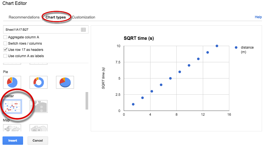
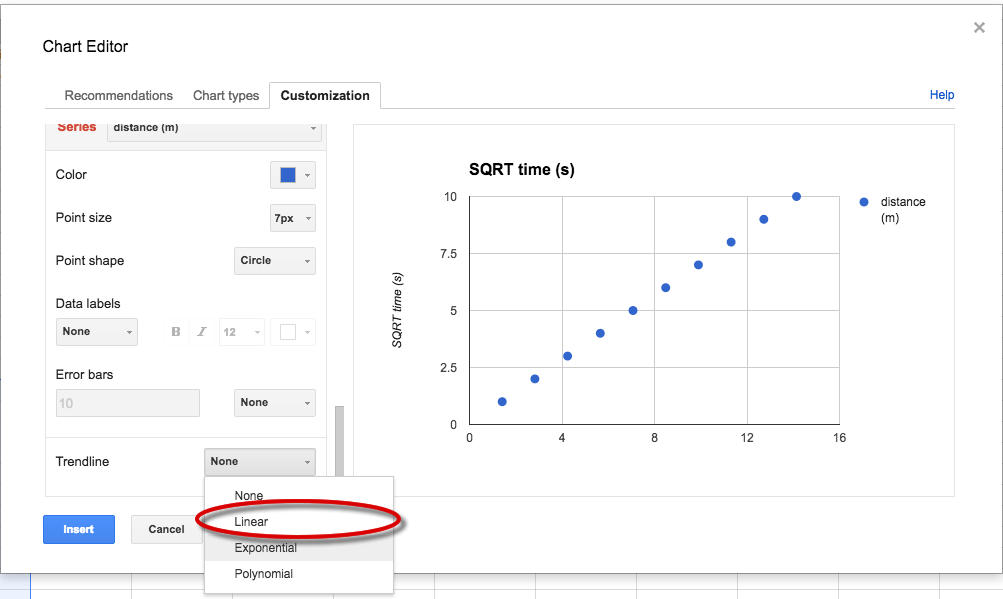
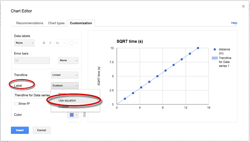
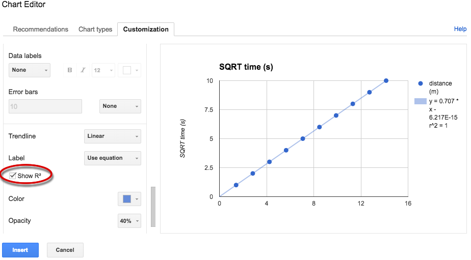
Written instructions for finding a "trendline" in Google Sheets.

1	Make sure each column has a header.
2	The independent data is in the left column and the dependent data is in the right column.
3	Highlight both columns of data, including the header,to be graphed.
4	From Google's "Insert"menu select "chart."
5	From the shart types menu select "scatter"
5	Assuming your data looks linear, go to the "Customization" tab in the "Chart Editor's" window.
6	There is a scrolling window in the left side of this dialog box. Scroll down until you see a command called "tredline."
7	There is a drop down buttom next to where it says trendlind. From this button choose "linear.
8	Underneath the trendline command is a title that says "Label." To the left of this is a drop down button. Click on it and select "Use equation."
9	Underneath all of this is a check box that says Show R². Check this box.
10	Click on the "Insert" button in the dialog box. To the right of the graph is hte trandline equationand R².

Below is a video showing how to use Google's Sheets Linearize data by finding the trendline

This video can be found on YouTube at https://youtu.be/F1jP_8y6nPc

by Tony Wayne ...(If you are a teacher, please feel free to use these resources in your teaching.)

The owner of this website does not collect cookies when the site is visited. However, this site uses and or embeds Adobe, Apple, GoDaddy, Google, and YouTube products. These companies collect cookies when their producs are used on my pages. Click here to go to them to find out more about how they use their cookies. If you do not agree with any of their policies then leave this site now.